CS184/284A Spring 2025 Homework 3 Write-Up
Names: Kenny Wang, Harris Thai
Link to webpage:
https://kilowatt.github.io/cs184/3/index.html
Link to GitHub repository:
Sweet Baby Rays
 Bunny! <3
Overview
In this assignment, our work very much built on top of itself. We implemented a large part of a rendering pipeline, starting with having rays sample the scene and detecting where they intersect primitives like triangles and spheres. We then implement a way to do this efficiently with Bounding Volume Hierarchies that split the mesh in a binary tree fashion to dramatically speed up the process of finding an intersection. We move on to direct lighting with zero-bounce illumination and then one-bounce illumination with both hemisphere and importance sampling on light sources. Naturally, we implement N-bounce lighting, or global illumination, and we implement a simple but effective technique for reducing computation time: Russian Roulette. Finally, we implement a highly effective yet still fast optimization called Adaptive Sampling, which samples rays until its value converges or it hits num_samples, whatever comes first. We learned a lot from completing this assignment, from the relatively simple math of intersections and pointer manipulation for constructing a BVH space efficiently, to the conceptually challenging but rewarding task of illuminating a point in space, first from light sources and extending our understanding to further bounces of light, all wrapped up nicely with a statistically satisfying adaptive sampling algorithm.
Part 1: Ray Generation and Scene Intersection
In the rendering pipeline, we start raytracing by dividing up the scene into tiles and then calling raytrace_pixel() for each pixel inside its extent. This function generates rays pointing out of the camera to detect what needs to be considered when rendering the pixel. The primitive intersection functions are useful to determine what surfaces these rays are incident upon.
Triangle Intersection Algorithm
The triangle intersection algorithm we implemented was the Möller-Trumbore intersection algorithm. This algorithm uses the points of a triangle to calculate edges, and uses those edges along with the ray origin and direction to calculate the time t at which it intersects, as well as the barycentric coordinates at which it does.
Sphere Intersection Algorithm
We implemented the sphere intersection algorithm from the lecture slide, where we use the ray origin direction as well as the radius and center of the sphere to calculate quadratic coefficients. Solving this quadratic equation, we get either 0, 1, or 2 real, unique values of t, which we make sure is at least 0 to confirm that it happens on the direction of the ray, not in the opposite direction.
Some Renders
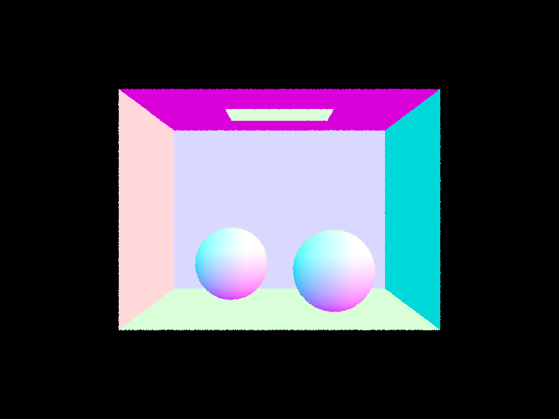 Spheres
|
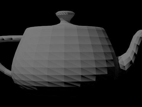
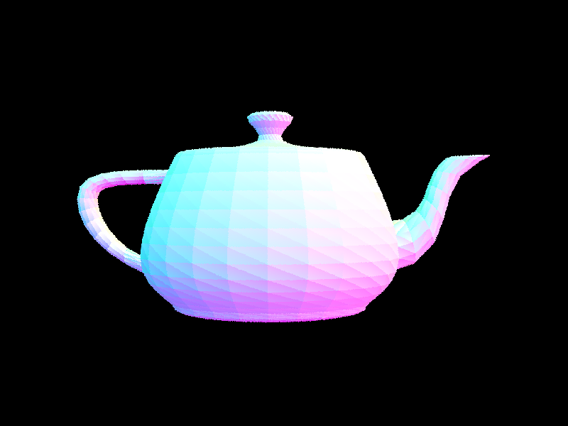 Teapot
|
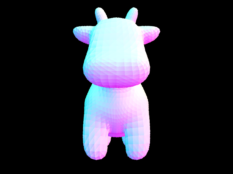 Cow
Cow
|
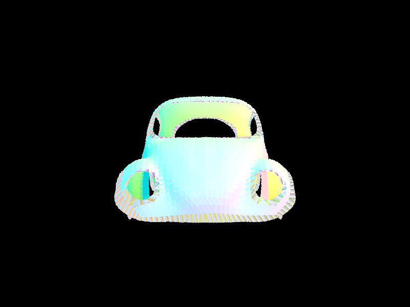 Beetle
|
Part 2: Bounding Volume Hierarchy
BVH Construction Algorithm
We start by calculating the bounding box that encompasses all the primitives and create a BVHNode for this BBox. We then calculate the longest side of the box based on its extent vector, and sort the primitives by their position along this maximum length axis. We then split by median by setting the start and end of the node's left and right primitives such that it splits the parent’s primitive vector in half by number of elements. Changing the pointers to form subvectors also has the benefit of being space-efficient.
A few more complex basic renders:
 Bunny
Bunny
|
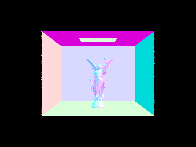 Lucy
Lucy
|
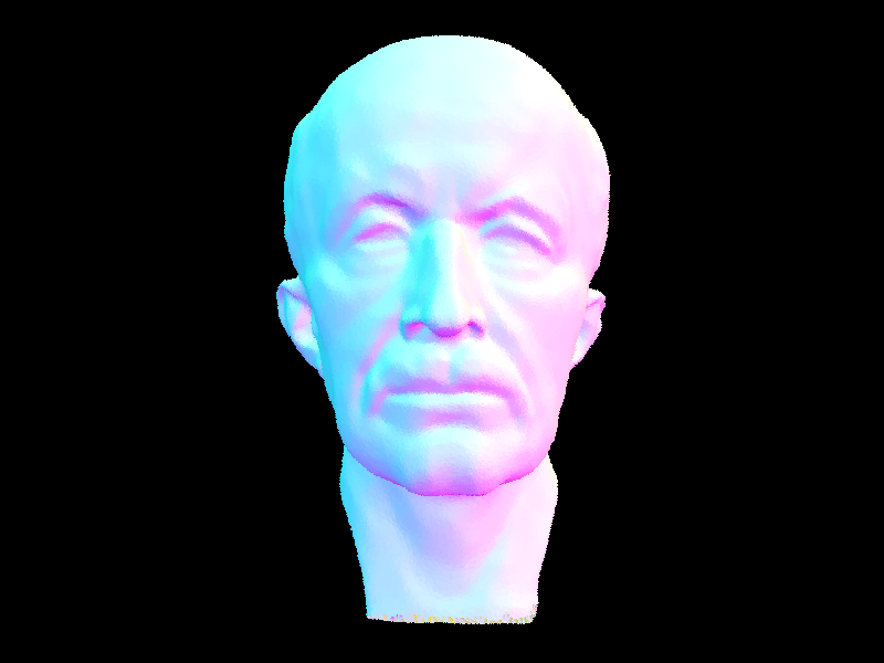 Max Planck
|
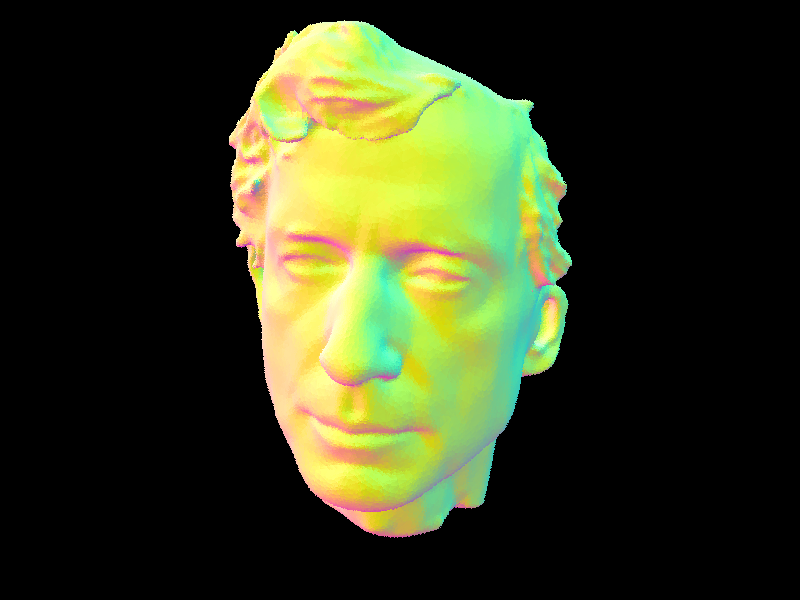 Peter
Peter
|
BVH Timing Analysis
Using BVH gives us an enormous speedup in rendering! Here's some numbers. Note that building the BVH takes time too, but this is negligible, especially compared to the savings. Without BVH, we need to run an O(N) check for every primitive, for each ray. Using BVH, we can cut that to O(log(N)) instead.
|
File
|
No BVH
|
With BVH
|
|
Teapot
|
6.7
|
0.19
|
|
Cow
|
17.2
|
0.17
|
|
Banana
|
3.6
|
0.14
|
|
Max Planck
|
498.6
|
0.56
|
Part 3: Direct Illumination
Uniform Hemisphere Sampling
For our hemispheric direct lighting function, we sampled from a hemisphere, converted it into worldspace coordinates, and constructed a ray pointed in that direction starting at hit_p. Setting the min_t of the ray to EPS_F, we check for its first intersection with the BVH tree and find the emission of the BSDF at that new sampled intersection point. We complete the calculation by getting the BSDF's reflectance at hit_p from the camera w_out to the sample wi (this is backwards to the actual direction of light but it is symmetrical) and the cosine of the incident angle, represented by wi in local space multiplied by the normal vector in object space (0, 0, 1). We multiply the reflectance by the incident emission and the cosine wi[2], divide by the pdf (1/(2pi)), and take an average across num_samples iterations to get the final result.
Importance Sampling
For our importance sampling direct lighting function, we iterate across the set of all lights and take samples from each, once if it is a delta light and ns_area_light times otherwise. When considering the contribution of each light source, we set the sample ray's max_t to distToLight - EPS_F and skip the sample if the ray has any valid intersection with an object before it intersects with the light. We finish the function in largely the same way as hemispheric sampling, except we divide by the pdf provided by each light's sample_L function instead of a constant value.
Hemisphere vs Importance Sampling
Hemisphere sampling is a bit of a naive approach, and importance sampling both saves time and improves the quality of our images.
 Bunny, Importance Sampling
|
 Bunny, Hemisphere Sampling
|
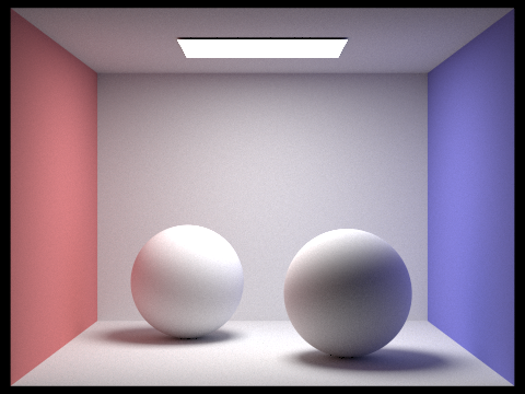
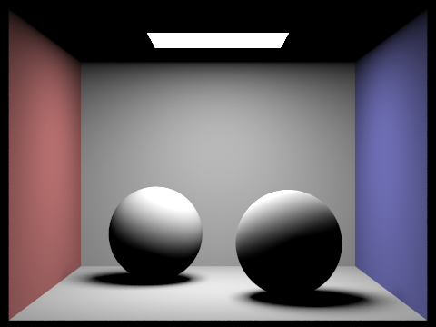 Spheres, Importance Sampling
|
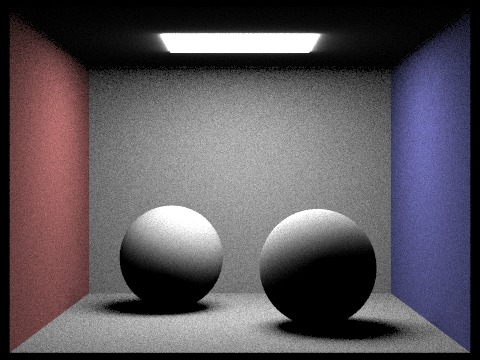 Spheres, Hemisphere Sampling
|
Effect of Number of Light Samples on Importance Sampling
Notice that more samples per light when importance sampling lights makes our renders less grainy. Here S = 1, so we use 1 camera ray per pixel, and we modify L, the number of samples per area light.
 L = 1
L = 1
|
 L = 4
L = 4
|
 L = 16
|
 L = 64
|
Part 4: Global Illumination
Indirect Lighting Algorithm
We implement indirect lighting by first setting each ray's depth to max_depth in raytrace_pixel(). In the at_least_one_bounce_radiance function, if the ray's depth is greater than 1, we use sample_f() to get a BSDF reflectance value, a sample direction in worldspace wi, and a pdf value. We create a ray pointing from hit_p in the direction of wi with a depth of r.depth - 1 and we only continue computation if this sample ray survives the termination probability and intersects with another object. At that point, we call the function recursively on this sample ray and new intersection and add the incoming radiance, divided by the survival probability, to L_out. If the ray's depth is equal to 0 or isAccumBounces is true, we also add the result of the one_bounce_radiance function on the current ray and intersection. In est_radiance_global_illumination, we add the result of at_least_one_bounce_radiance to zero_bounce_radiance to get our final result.
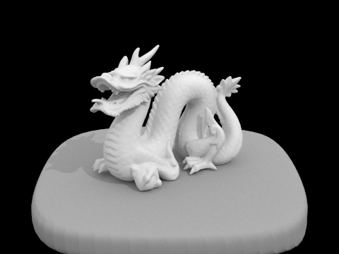
Nice Renders
|
Bunny
|
 Spheres
|
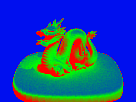
 Dragon
|
 Teapot
|
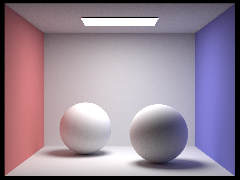
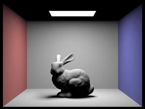
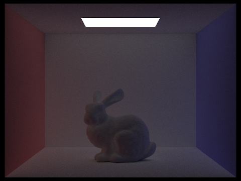
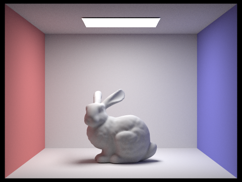
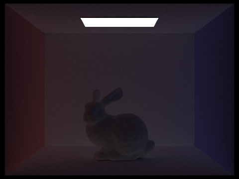
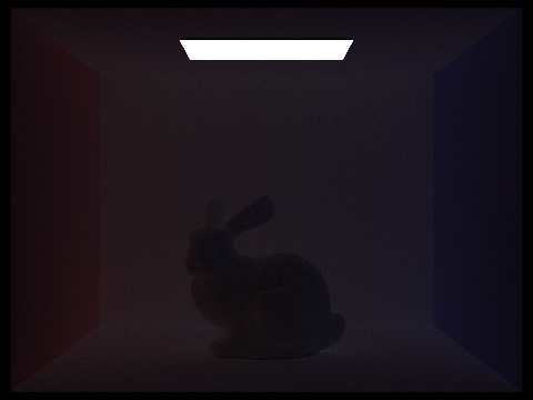
Direct vs Indirect Illumination
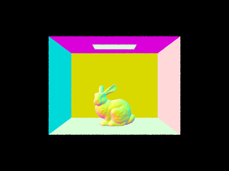
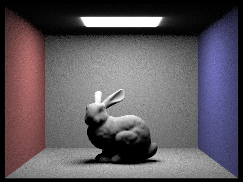
Here is CB Bunny with only direct illumination, and then only indirect illumination. We can see that with only direct illumination, we have hard shadows and no light reaching the ceiling.
 Direct Lighting Only
|
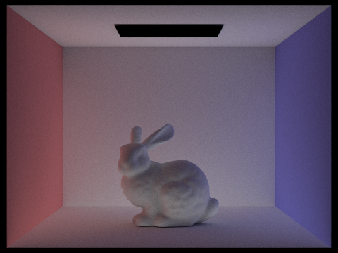 Indirect Lighting Only
|
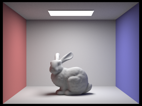
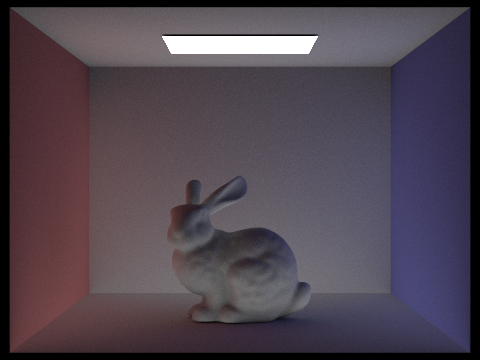
Effects of Ray Depth
Changing the value of M, for max ray depth, and toggling bounce accumulation lets us visualize the effect of each successive bounce. Notice how each successive bounce gets less and less bright, so we don't need more than about 5 bounces to get a great image.
 M = 0
M = 0
|
M = 0, no accumulate
|
 M = 1
M = 1
|
 M = 1, no accumulate
|
 M = 2
M = 2
|
 M = 2, no accumulate
|
 M = 0
M = 0
|
 M = 0, no accumulate
|
 M = 0
M = 0
|
 M = 0, no accumulate
|
|
M = 0
|
 M = 0, no accumulate
|
Russian Roulette
Using the Russian Roulette technique allows us to estimate infinite bounces without bias. For some reason, you guys want us to limit it to a set number of bounces, which kind of defeats the point. Observe how we can set M really high (like 100), and it will still run in a very reasonable amount of time.
|
M = 0
|
M = 1
|
|
M = 2
|
M = 3
|
|
M = 4
|
 M = 100
|
Effect of Per-Pixel Sample Rate
We can see that higher S, meaning more samples per pixel, leads to less grainy images. Here we set L = 4, so we have 4 rays per area light, and M = 5, so 5 max bounces. S = 1024 is really pretty, so we'll use it for a lot of our other renders.
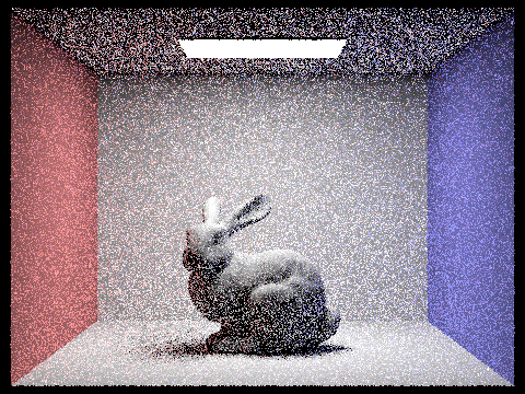 S = 1
S = 1
|
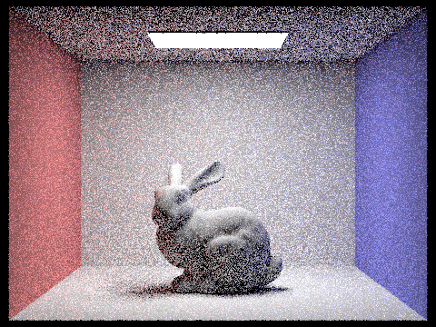 S = 2
S = 2
|
 S = 4
S = 4
|
 S = 8
S = 8
|
 S = 16
|
 S = 64
|
|
S = 16
|
S = 64
|
|
S = 1024
|
Part 5: Adaptive Sampling
Adaptive sampling attempts to not waste samples on pixels whose render values converge quickly, instead focusing computation on trickier pixels. As a result, we sample until we reach num_samples or the convergence I is at most maxTolerance times the mean. We check this condition every samples_per_batch iterations except for the first. We calculate the mean and the var by storing the sum of the illuminances s1, the sum of the squared illuminances s2, and the number of iterations so far.
Take note of how adaptive sampling focuses on shadows and poorly-lit areas.
 Bunny
Bunny
|
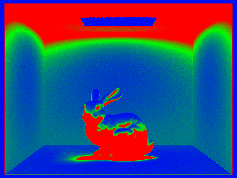 Rate
Rate
|
 Spheres
|
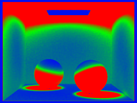 Rate
Rate
|
 Dragon
|
 Rate
Rate
|