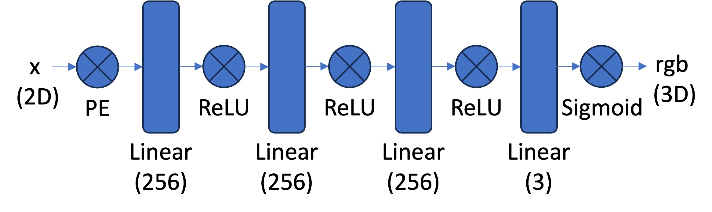
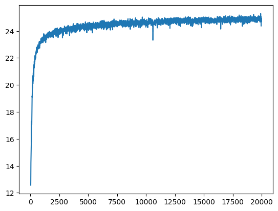
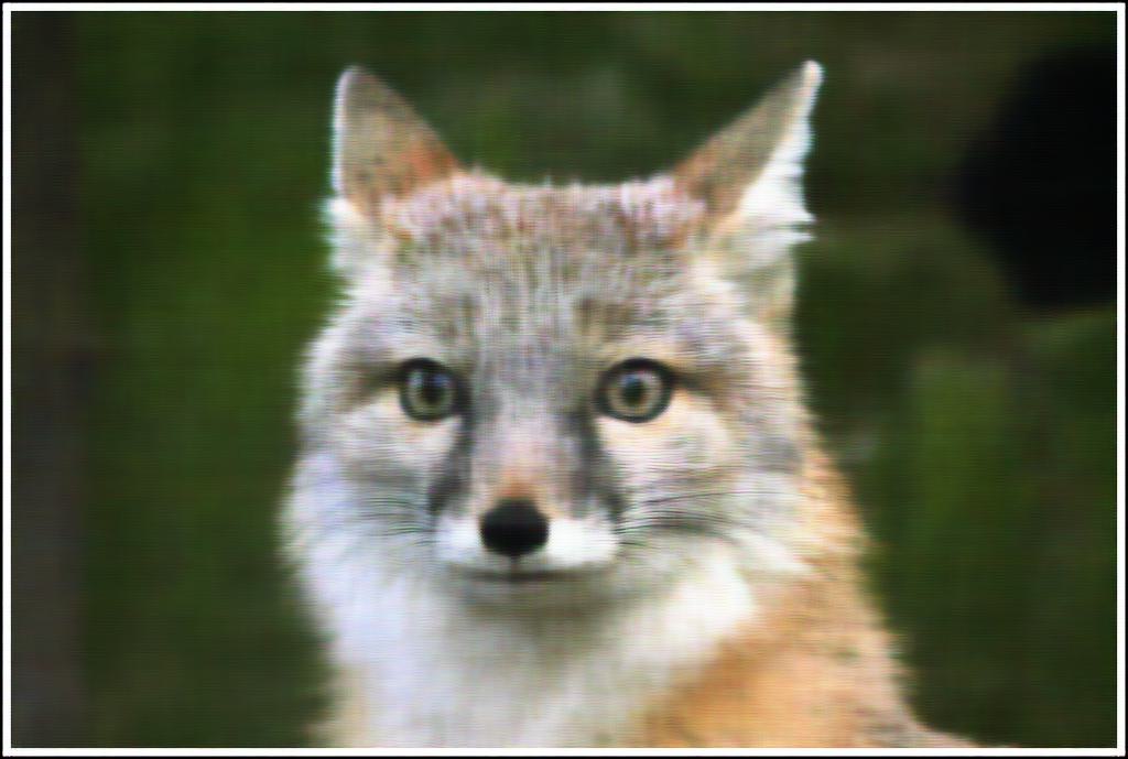
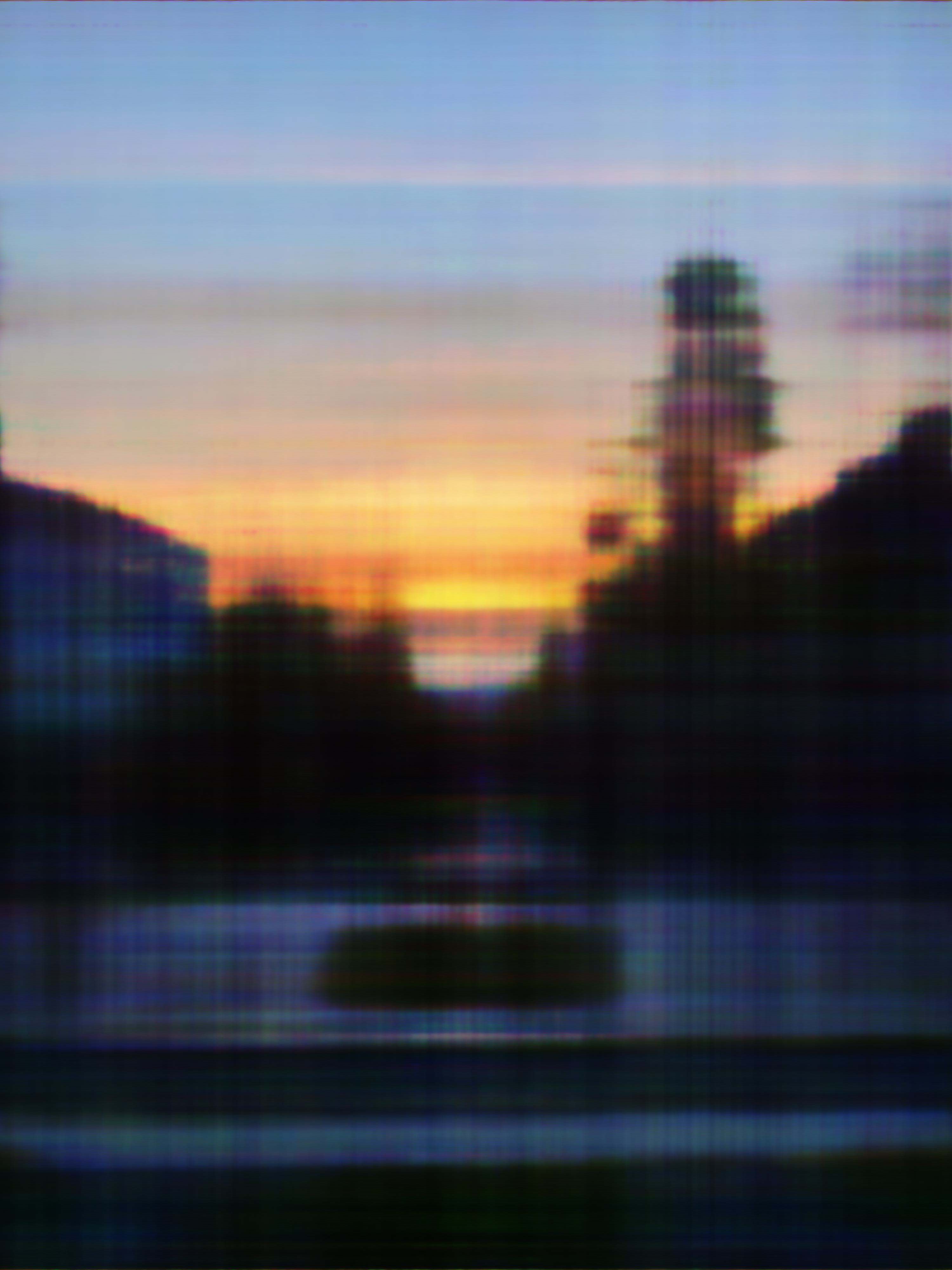
lr=1e-2, and MSE loss. Training until 20k epochs only takes about 1 minute!
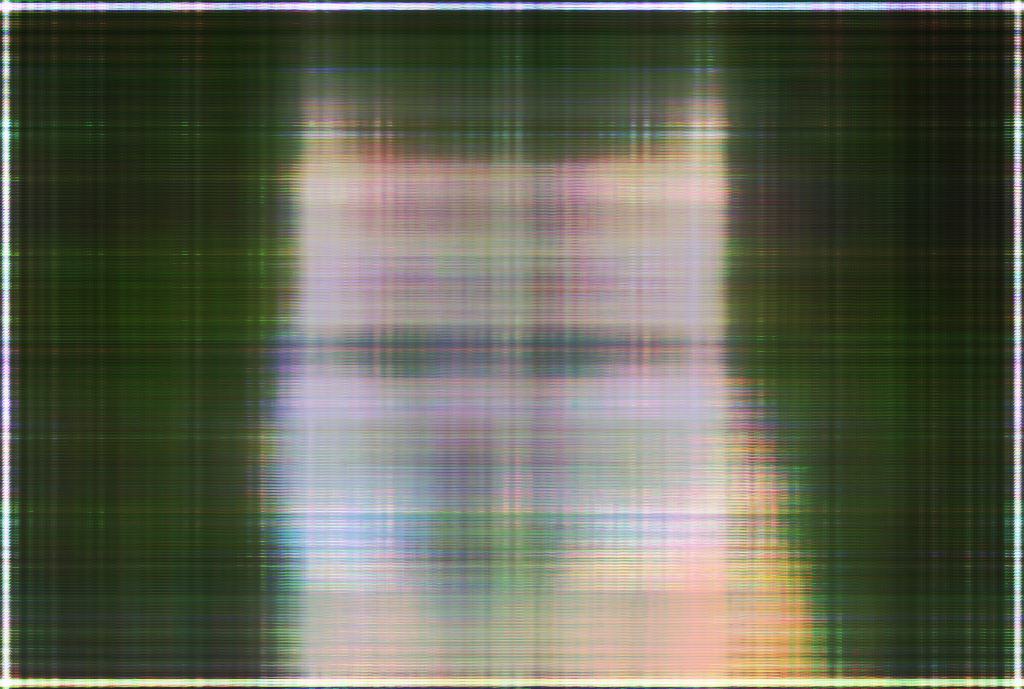
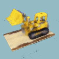
100 epochs
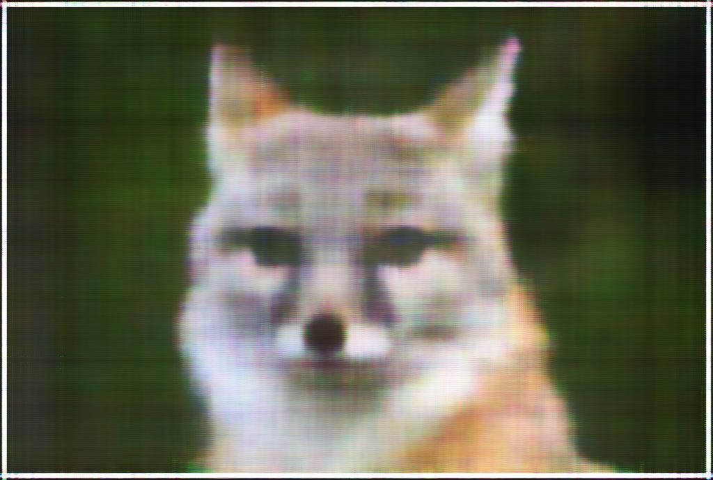
500 epochs
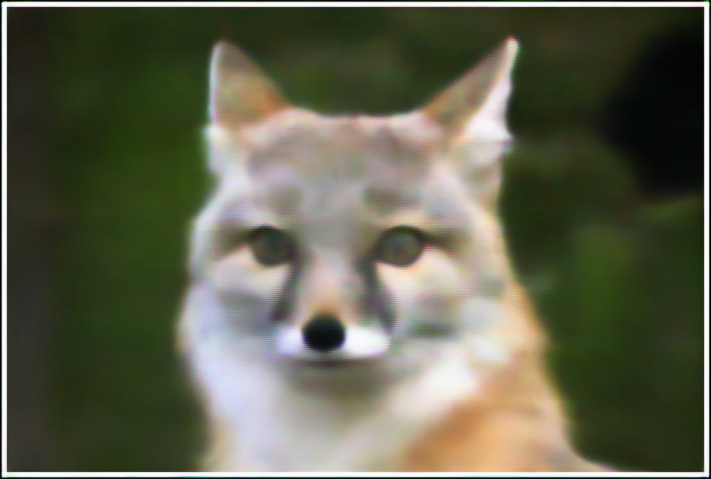
20k epochs
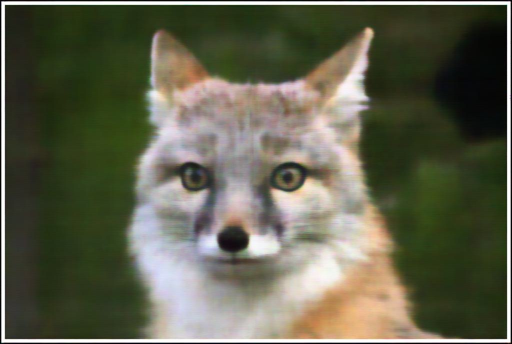
Original
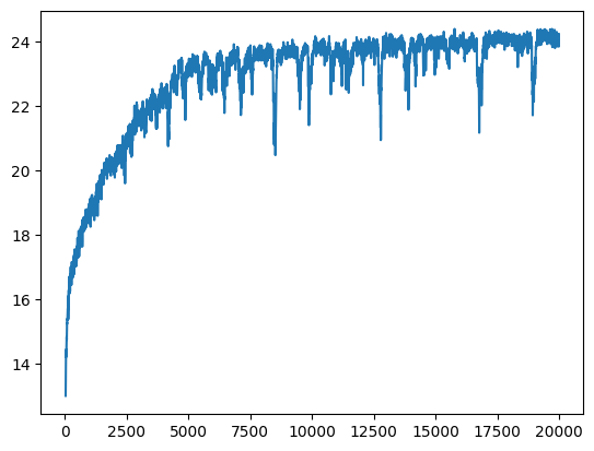
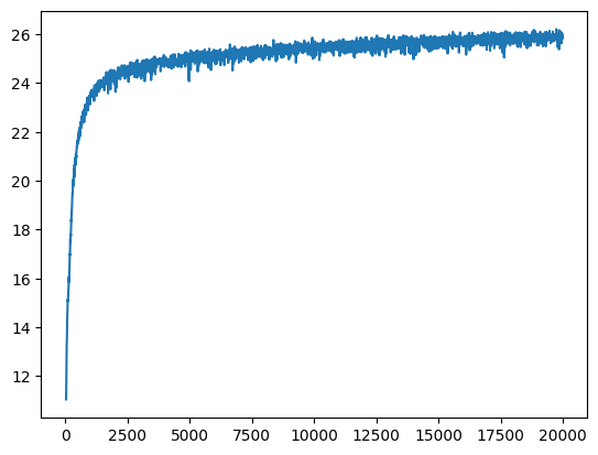
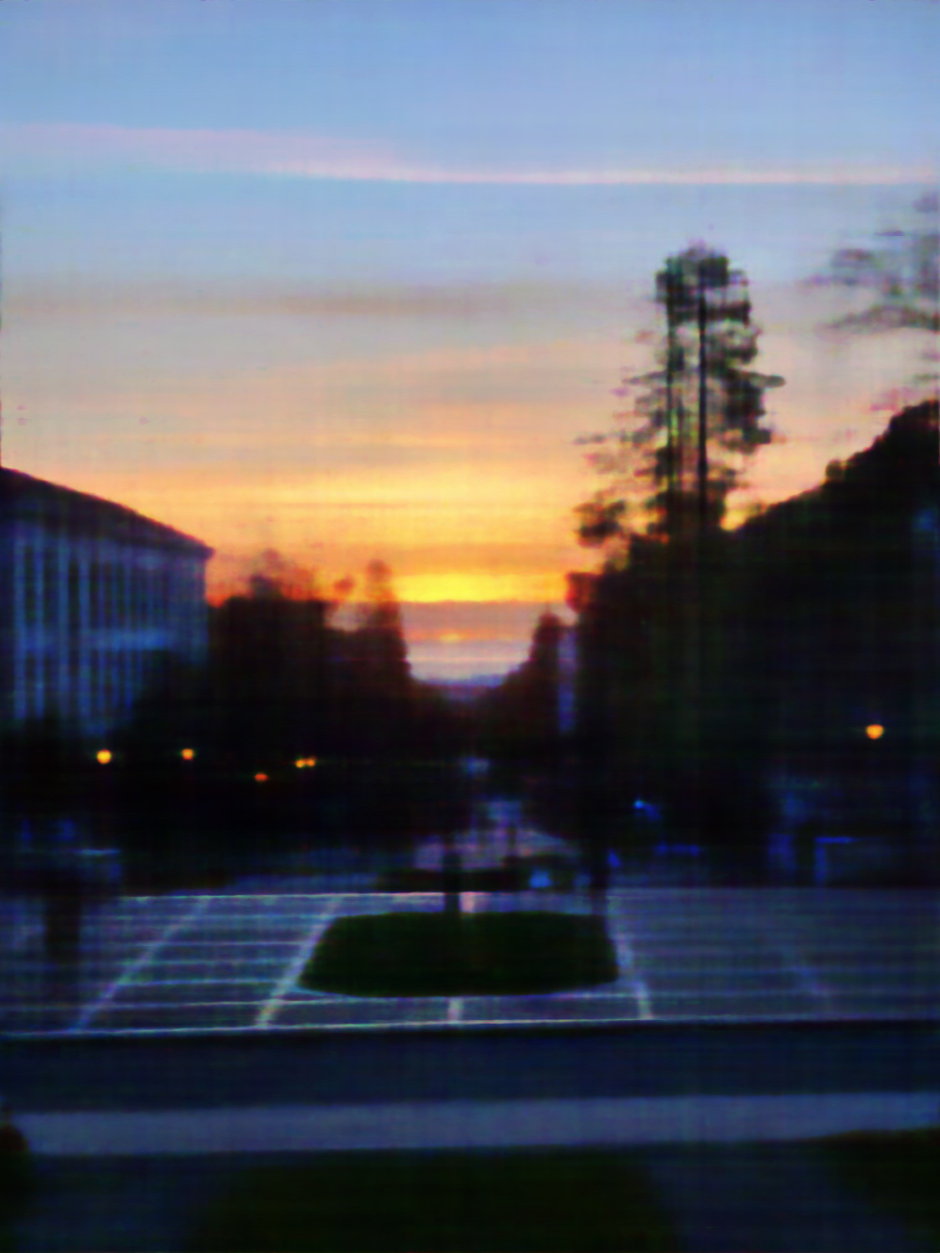
L=5 instead of 10 for the positional encoding, which we can see is worse. Another is using lr=1e-3 instead of lr=1e-2, which is actually ... better than the standard params!!
L=5
Standard Params
lr=1e-3
Original
L=5
Standard Params
lr=1e-3
100 epochs
500 epochs
20k epochs
Original
x_w = transform(c2w, x_c), which takes in batched 3D camera coordinates x_c and a 4x4 camera-to-world matrix c2w and outputs batched 3D world coordinates. This is a straightforward matrix multiplication, but internally, the function also converts to and from homogeneous coordinates.
x_c = pixel_to_camera(K, uv, s) takes in 3x3 intrinsic matrix K, batched 2D (u,v) pixel coordinates uv, and depth scalar s. It outputs the batched pixel coordinates converted into 3D camera coordinates. This involves just a bit of linear algebra.
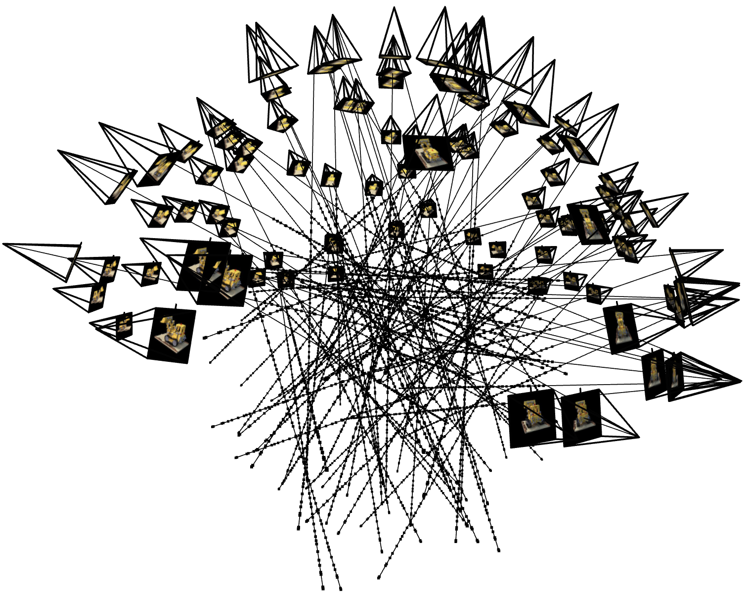
ray_o, ray_d = pixel_to_ray(K, c2w, uv) converts pixel (u,v) coordinates into the origin and direction of their associated 3D ray. The function takes in 3x3 intrinsic matrix K, batched 4x4 camera-to-world matrices c2w, and batched 2D (u,v) pixel coordinates uv. It outputs ray_o, the 3D origin vector, and ray_d, the 3D direction vector of the ray.
RaysData class to act as a dataloader, taking as parameters the intrinsic matrix K, a collection of images imgs, and the corresponding 4x4 camera-to-world matrices c2ws. It stores all the pixels in its set of images into one long flattened array, and has the method sample_rays. This method randomly selects batch_size pixels from the entire set of images, returning ray_o and ray_d, representing the rays for each of those pixels, and rgb, the RGB pixel values. This sampling function uses the helper functions we created earlier.
sample_along_rays, which takes in ray_o and ray_d to represent a batch of rays. It then outputs the 3D coordinates of 64 points along each ray between distances 2.0 and 6.0. The optional perturb parameter determines whether to add slight randomness to the otherwise evenly-spaced points, and is useful for training.
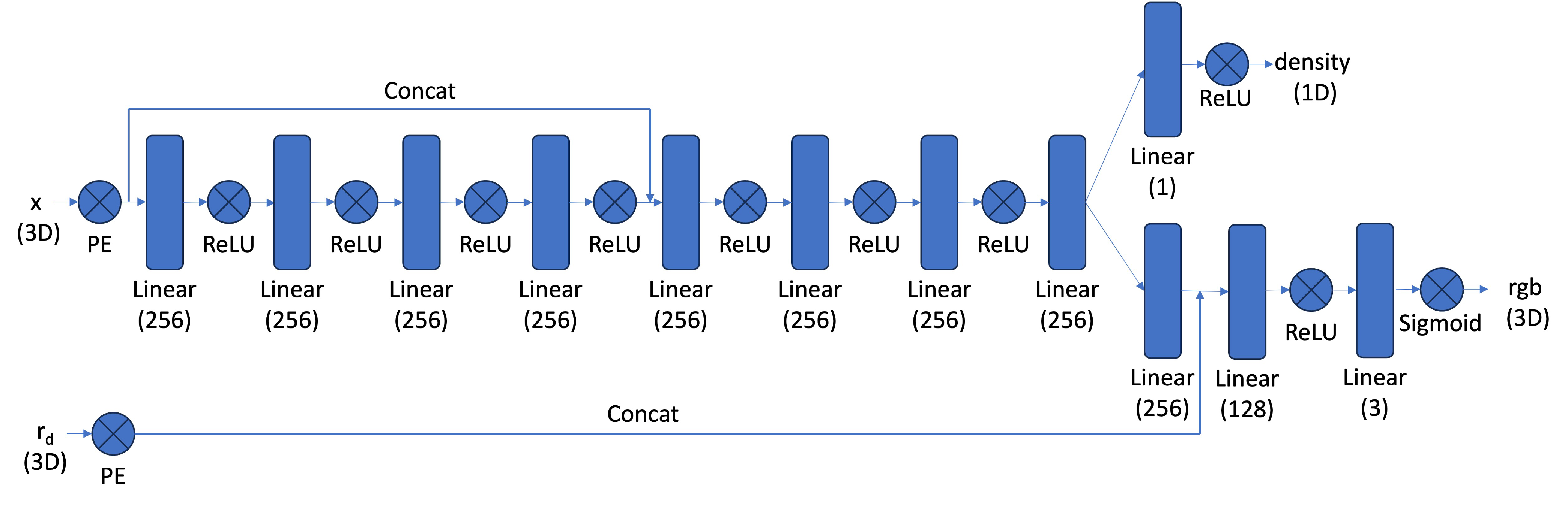
lr=5e-4.
volrend(sigmas, rgbs, step_size) which takes in batched densities sigmas, batched RGB pixel values rgbs, and the distance between points in the ray step_size. The function outputs the final observed RGB pixel value.
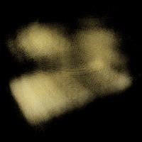
100 epochs
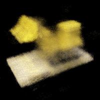
200 epochs
500 epochs
1k epochs

10k epochs

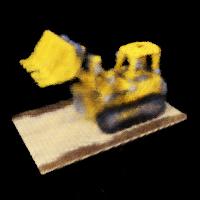
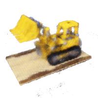
30k epochs
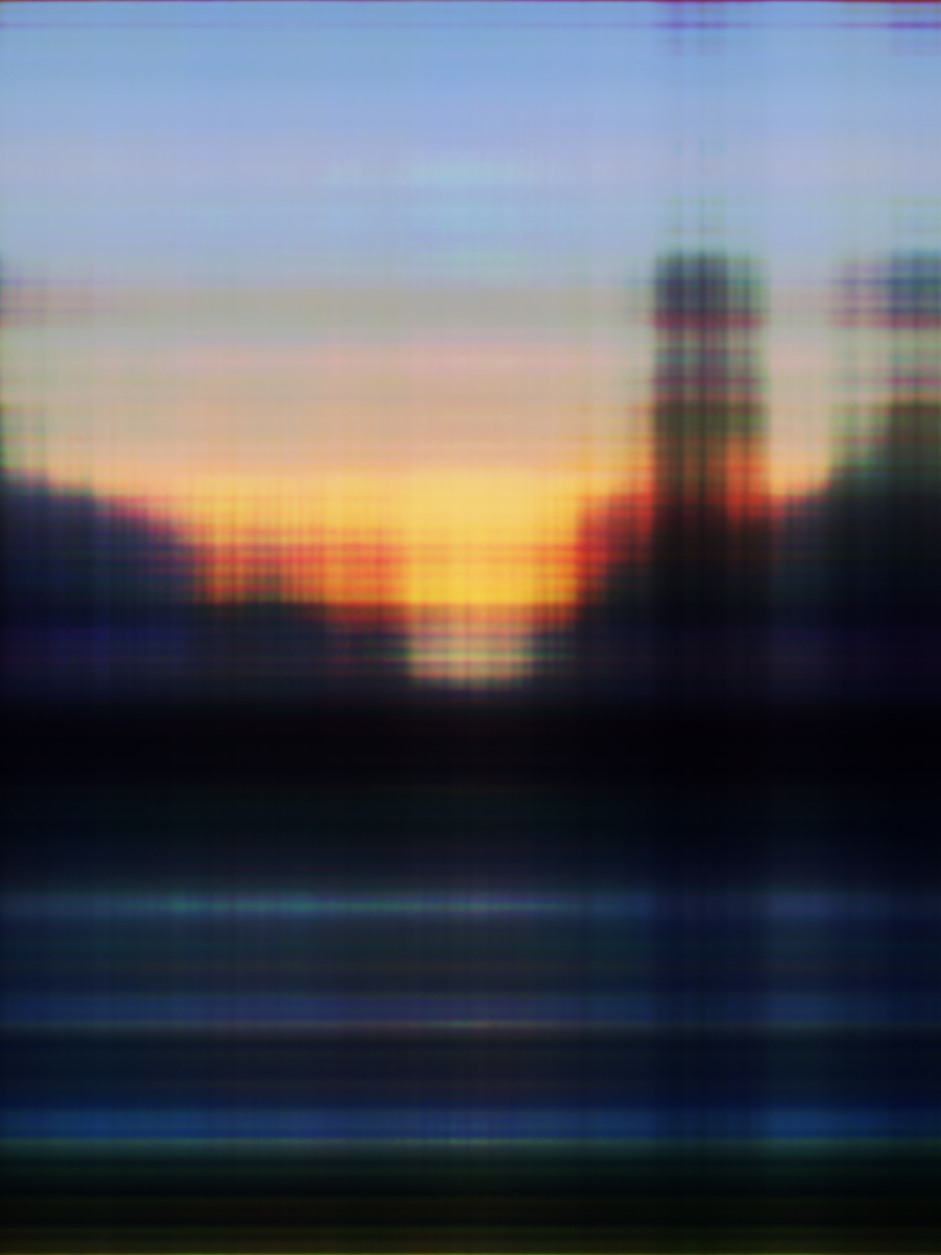
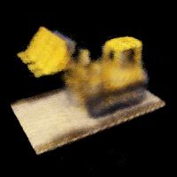
1k epochs (< 20 minutes)
30k epochs (~9 hours)

Acknowledgements |